Surface can reflect beam from lidar.
factors that influence reflectivity
Surface Properties
- Material Reflectivity (Albedo)
- Color
- Surface Roughness (Texture)
- Surface Orientation (Incident Angle)
| Factor | Effect on Intensity |
|---|---|
| Surface color | Dark → Low; Bright → High |
| Material reflectivity | High albedo → High intensity |
| Texture / roughness | Smooth → High; Rough → Low |
| Angle of incidence | Perpendicular → High |
| Distance to target | Farther → Lower intensity |
| Atmospheric interference | Fog/dust → Lower intensity |
| LiDAR wavelength | Depends on material response |
| Sensor power & sensitivity | Higher → Stronger returns |
note:
- Color ≠ reflectivity in all cases. Two objects of different visible colors might still have similar infrared reflectivity, depending on their pigment chemistry.
- Empirical testing or manufacturer data is often required to know exact reflectivity values at specific wavelengths.
LiDAR Sensor Characteristics
- Wavelength: The reflectivity of surfaces varies with wavelength.
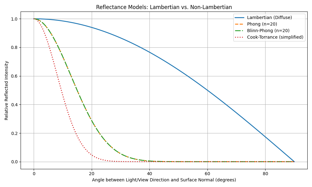
reflectance models
| Reflectance Type | example | Effect When direction of light and viewpoint are the same |
|---|---|---|
| Lambertian | unpolished chalk | No change — still view-independent |
| Phong | polished plastic or wood with a shiny coating | Specular highlight is maximized |
| Blinn-Phong | Specular term maximized (via halfway vector) | |
| Cook-Torrance | brushed metal, skin, or real-world materials under realistic lighting | Strong specular peak (especially at oblique angles) |
 .
.
Here is a picture for reflectance models. A python script to generate this image is provided below.
import numpy as np
import matplotlib.pyplot as plt

# Define angles from 0 to 90 degrees (converted to radians)
theta_deg = np.linspace(0, 90, 500)
theta_rad = np.radians(theta_deg)

# Lambertian: Intensity ~ cos(theta)
lambertian = np.cos(theta_rad)

# Phong: Specular ~ cos(theta)^n, assume n = 20 for shiny surface
n_phong = 20
phong_specular = np.cos(theta_rad) ** n_phong

# Blinn-Phong: also uses cos(theta)^n; here we approximate similar behavior
# This assumes halfway vector H close to the normal; use same exponent for comparison
blinn_phong_specular = np.cos(theta_rad) ** n_phong

# Cook-Torrance (simplified model): peak at grazing angles
# We'll model a simplified specular peak near 0 degrees (oblique incidence)
cook_torrance = np.exp(-((theta_rad - 0) / 0.2)**2)  # Gaussian centered at 0 rad

# Plot all
plt.figure(figsize=(10, 6))
plt.plot(theta_deg, lambertian, label='Lambertian (Diffuse)', linewidth=2)
plt.plot(theta_deg, phong_specular, label='Phong (n=20)', linestyle='--', linewidth=2)
plt.plot(theta_deg, blinn_phong_specular, label='Blinn-Phong (n=20)', linestyle='-.', linewidth=2)
plt.plot(theta_deg, cook_torrance, label='Cook-Torrance (simplified)', linestyle=':', linewidth=2)

plt.xlabel('Angle between Light/View Direction and Surface Normal (degrees)')
plt.ylabel('Relative Reflected Intensity')
plt.title('Reflectance Models: Lambertian vs. Non-Lambertian')
plt.legend()
plt.grid(True)
plt.tight_layout()
plt.show()
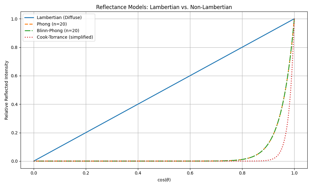
Here is a picture to describe curve between cosine and reflectivity for reflectance models and python script is provide, too.
 .
.
import numpy as np
import matplotlib.pyplot as plt

# Define angles from 0 to 90 degrees (converted to radians)
theta_deg = np.linspace(0, 90, 500)
theta_rad = np.radians(theta_deg)

# Compute cos(theta) for x-axis
cos_theta = np.cos(theta_rad)

# Lambertian: Intensity ~ cos(theta)
lambertian = cos_theta

# Phong: Specular ~ cos(theta)^n, assume n = 20 for shiny surface
n_phong = 20
phong_specular = cos_theta ** n_phong

# Blinn-Phong: similar form, using same exponent
blinn_phong_specular = cos_theta ** n_phong

# Cook-Torrance (simplified): peak at grazing angles (theta = 0 -> cos(theta) = 1)
cook_torrance = np.exp(-((theta_rad - 0) / 0.2)**2)  # Gaussian centered at 0 rad

# Plot all
plt.figure(figsize=(10, 6))
plt.plot(cos_theta, lambertian, label='Lambertian (Diffuse)', linewidth=2)
plt.plot(cos_theta, phong_specular, label='Phong (n=20)', linestyle='--', linewidth=2)
plt.plot(cos_theta, blinn_phong_specular, label='Blinn-Phong (n=20)', linestyle='-.', linewidth=2)
plt.plot(cos_theta, cook_torrance, label='Cook-Torrance (simplified)', linestyle=':', linewidth=2)

plt.xlabel(r'$\cos(\theta)$')
plt.ylabel('Relative Reflected Intensity')
plt.title('Reflectance Models: Lambertian vs. Non-Lambertian')
plt.legend()
plt.grid(True)
plt.tight_layout()
plt.show()
While intensity values can match, they do not mean the surfaces are the same. This is why raw LiDAR intensity is not reliable alone for material or surface classification.
intensity and angle
| Surface Type | 0° (Normal) | ~45° | ~80° | Characteristic Pattern |
|---|---|---|---|---|
| Lambertian | High | Medium | Low Cosine | decay |
| Specular | Low | Low | High only if sensor = specular | Sharp peak at specular angle |
| Diffuse + Specular Mix | High | Medium | Bump | Cosine + spike |
| Retroreflective | High | High | High | Flat or inverted V |
| Subsurface Scatter | High | Medium | Medium | Gentle decline |
for asphalt
- The fall-off may be less smooth.
- There may be small fluctuations in return intensity even for fixed angle and distance.
- The surface acts like a low-brightness diffuse scatterer.
Some materials may look similar to the human eye (in visible light) but have very different reflectivity in the infrared, vice versa.